Tutorial for CCC-RISE: Cell-Cell Communication Analysis

This tutorial demonstrates the complete CCC-RISE workflow for analyzing cell-cell communication in single-cell RNA-seq data across experimental conditions.

Installation

To add CCC-RISE to your Python package, add the following line to your requirements.txt and remake your virtual environment:

git+https://github.com/meyer-lab/cellcommunication-Pf2.git@main

Preprocessing the Dataset

Input Requirements

Your AnnData object must meet the following requirements:

1. Condition Index: Include an observations column condition_unique_idxs that is a 0-indexed array indicating which condition each cell is derived from, along with the cell barcode. Condition 1 cells are indexed as 0, Condition 2 as 1, and so on.

2. Preprocessing: Your AnnData object must be preprocessed (doublets removed, genes filtered, normalized, and log-transformed) before running CCC-RISE. Standard preprocessing functions can assist with gene filtering, normalization, and assigning condition_unique_idxs.

Ligand-Receptor Pairs

CCC-RISE requires a DataFrame of ligand-receptor pairs to analyze cell-cell communication. This can be obtained from resources like CellChat or other ligand-receptor databases.

Required DataFrame Format:

• Must contain columns named ligand and receptor

• Gene names should match those in your AnnData object (typically uppercase)

• For protein complexes, subunits should be separated by & (e.g., CD74&CD44)

• Example structure:

  ligand     receptor
  CCL19      CCR7
  PTN        PTPRZ1
  CD74&CD44  CD44
  

The package includes a default function import_ligand_receptor_pairs() that loads a curated database from CellChat, but you can provide your own DataFrame following this format.

Import and Prepare the Dataset

The prepare_dataset function assists with preprocessing your data. Parameters:

• X: AnnData object containing raw count data in sparse matrix format

• condition_name: Name of the column in X.obs that specifies experimental conditions for each cell

• geneThreshold: Minimum mean expression threshold for gene filtering (genes with mean expression below this value are removed)

• deviance: If True, applies deviance transformation instead of log normalization (default: False)

The function performs the following steps:

• Filters cells with fewer than 10 total counts

• Filters genes based on the geneThreshold parameter

• Normalizes total counts per cell to the median

• Scales gene expression values

• Applies log₁₀((1000 × normalized_value) + 1) transformation (or deviance transformation if specified)

• Creates condition_unique_idxs column in X.obs with 0-indexed condition assignments

• Pre-calculates gene means and stores in X.var["means"]

Example Code:

Import your dataset as an AnnData object with preprocessed data:

from cellcommunicationpf2.import_data import prepare_dataset, import_ligand_receptor_pairs
import anndata

# Load your data
X = anndata.read_h5ad("your_data.h5ad")

# Prepare the dataset
X = prepare_dataset(X, condition_name="condition", geneThreshold=0.01)

# Load ligand-receptor pairs
lr_pairs = import_ligand_receptor_pairs()

Choosing the Rank

CCC-RISE involves two sequential factorization steps, each requiring rank selection:

1. RISE Rank Selection: Determines how many components to extract from the raw scRNA-seq data

2. CPD Rank Selection: Determines how many components to use when factorizing the interaction tensor

Both steps require careful evaluation using two complementary metrics:

• R²X (Variance Explained): Measures the proportion of variance in the data explained by the model. Higher values indicate better model fit, but values plateau as rank increases, suggesting diminishing returns.

• FMS (Factor Match Score): Measures the stability/reproducibility of components across different random initializations or bootstrap samples. Values above ~0.6 indicate stable, reliable components. Low FMS suggests overfitting or noise.

RISE Rank Selection

What is RISE?

RISE (Reduction and Insight in Single-cell Exploration) is an unsupervised, tensor-based computational method designed for the integrative analysis of single-cell RNA sequencing (scRNA-seq) data across multiple experimental conditions, such as drug treatments, patient cohorts, or time points. Built upon the PARAFAC2 tensor decomposition framework, RISE preserves the inherent three-dimensional structure of multi-condition single-cell data—conditions × cells × genes—instead of flattening it into a conventional two-dimensional matrix. The RISE rank determines how many latent patterns are extracted before computing cell-cell communication scores.

Evaluate RISE Ranks

Test different RISE ranks to find the optimal balance between model complexity and stability:

from cellcommunicationpf2.figures.commonFuncs.plotGeneral import plot_fms_r2x_diff_ranks
import matplotlib.pyplot as plt

# Create figure with two subplots
fig, ax = plt.subplots(1, 2, figsize=(12, 4))

rise_ranks = list(range(5, 41, 5))

# Plot FMS and R2X for different RISE ranks
plot_fms_r2x_diff_ranks(
    X,
    condition_name="condition_unique_idxs",
    ax1=ax[0],
    ax2=ax[1],
    ranksList=rise_ranks,
    runs=e
)

ax[0].set_title('RISE: Factor Match Score (FMS)')
ax[0].set_xlabel('RISE Rank')
ax[1].set_title('RISE: Variance Explained (R²X)')
ax[1].set_xlabel('RISE Rank')
plt.tight_layout()
plt.show()

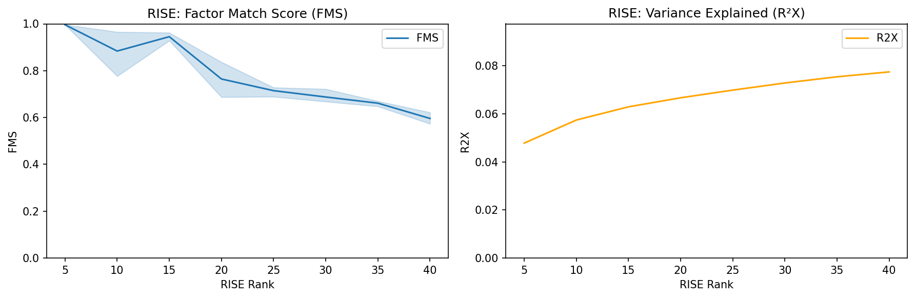
Interpretation:

• R²X: Look for where the curve begins to plateau. Beyond this point, additional components explain minimal additional variance.

• FMS: Choose a rank where FMS is above 0.6, indicating stable components. Higher FMS means the factors are more reproducible.

• Recommendation: Balance both metrics. Typically, select the rank where FMS exceeds 0.6 and R²X shows diminishing returns (e.g., RISE rank = 20-40 for most datasets).

CPD Rank Selection

What is CPD?

After RISE, an interaction tensor is computed from cell-cell communication scores between all cell pairs across L-R pairs and conditions. CPD (Canonical Polyadic Decomposition) factorizes this tensor to identify interpretable communication patterns. The CPD rank determines how many communication components are extracted.

Evaluate CPD Ranks

First, calculate the interaction tensor using a selected RISE rank, then test different CPD ranks:

from cellcommunicationpf2.tensor import calculate_interaction_tensor, run_fms_r2x_analysis
import seaborn as sns
import matplotlib.pyplot as plt

# Calculate interaction tensor with chosen RISE rank
rise_rank = 35  # Based on RISE analysis above
interaction_tensor = calculate_interaction_tensor(X, lr_pairs, rise_rank=rise_rank)

# Test CPD ranks
rank_list = list(range(1, 11, 2))
df = run_fms_r2x_analysis(
    interaction_tensor,
    rank_list=rank_list,
    runs=3,
    svd_init="random"
)

# Plot CPD FMS and R2X
fig, ax = plt.subplots(1, 2, figsize=(12, 4))

sns.lineplot(data=df, x="Component", y="FMS", ax=ax[0], label="FMS")
ax[0].set_ylim(0, 1)
ax[0].set_xlabel('CPD Rank')

sns.lineplot(data=df, x="Component", y="R2X", ax=ax[1], color="orange", label="R2X")
ax[1].set_ylim(0, np.max(df["R2X"]) + 0.02)
ax[1].set_xlabel('CPD Rank')

plt.tight_layout()
plt.show()

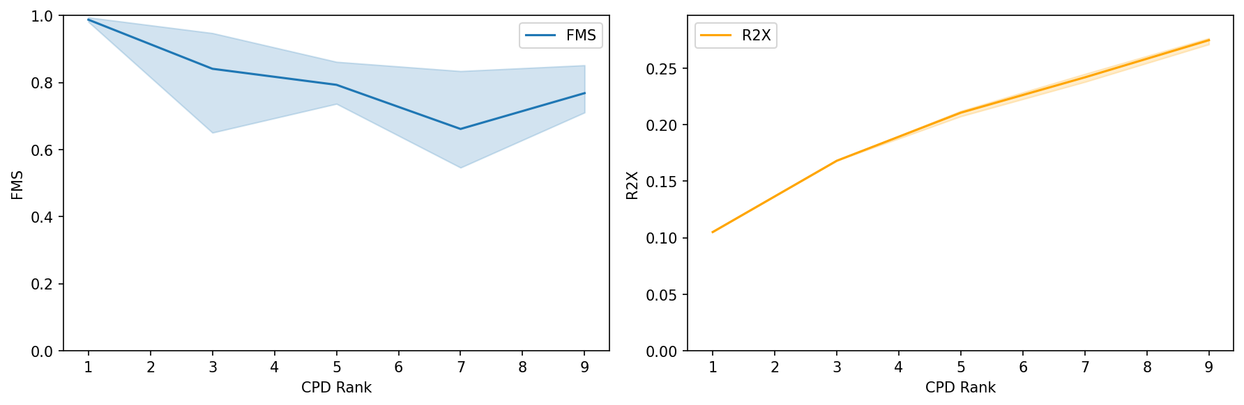
Interpretation:

• R²X: Monitor how much of the interaction tensor’s variance is explained. Look for an elbow point where additional components provide minimal improvement.

• FMS: Ensure components are stable (FMS > 0.6). Lower FMS indicates components may vary significantly with different initializations.

• Recommendation: Select the CPD rank where both FMS is high (>0.6) and R²X shows an elbow. Typically 5-20 components capture most meaningful communication patterns.

Running the Factorization

Perform CCC-RISE Factorization

Based on the rank selection analysis above, choose appropriate RISE and CPD ranks and run the complete CCC-RISE workflow. This performs the two-step factorization: first extracting latent communication modes from expression data (RISE), then factorizing the resulting interaction tensor (CPD):

from cellcommunicationpf2.tensor import run_ccc_rise_workflow

# Select ranks based on FMS/R2X analysis
rise_rank = 35  # Selected from RISE rank analysis
cp_rank = 8     # Selected from CPD rank analysis

# Run the complete workflow
X, r2x = run_ccc_rise_workflow(
    adata=X,
    rise_rank=rise_rank,
    cp_rank=cp_rank,
    lr_pairs=lr_pairs,
    condition_column="condition_column",
    n_iter_max=10000,
    tol=1e-9,
    random_state=42,
    complex_sep="&",
    doEmbedding=True
)

print(f"Variance Explained (R²X): {r2x:.4f}")

Function Parameters

The run_ccc_rise_workflow function executes the complete CCC-RISE pipeline:

• adata: AnnData object with preprocessed scRNA-seq data

• rise_rank: Number of PARAFAC2 components to extract from expression data

• cp_rank: Number of CPD components for factorizing the interaction tensor (if None, defaults to rise_rank)

• lr_pairs: DataFrame of ligand-receptor pairs with ‘ligand’ and ‘receptor’ columns

• condition_column: Column name in adata.obs containing condition identifiers (default: “sample”)

• n_iter_max: Maximum iterations for decomposition (default: 100)

• tol: Convergence tolerance (default: 1e-3)

• random_state: Random seed for reproducibility (default: None)

• complex_sep: Separator for protein complexes in L-R pairs (default: None)

• doEmbedding: If True, computes PaCMAP embeddings for visualization (default: True)

• svd_init: Initialization method for CPD (‘svd’ or ‘random’, default: ‘svd’)

What Gets Stored

The function returns the AnnData object with added results and the final R²X value. The following are stored in the AnnData object:

Factor Matrices (in X.uns):

• X.uns["weights"] - Component weights (array of length cp_rank)

• X.uns["A"] - Condition factor matrix (n_conditions × cp_rank)

• X.uns["B"] - Sender cell type factor matrix (rise_rank × cp_rank)

• X.uns["C"] - Receiver cell type factor matrix (rise_rank × cp_rank)

• X.uns["D"] - Ligand-receptor pair factor matrix (n_lr_pairs × cp_rank)

Cell Projections (in X.obsm):

• X.obsm["projections"] - Cell projections from PARAFAC2 (n_cells × rise_rank)

• X.obsm["sc_B"] - Sender cell loadings (n_cells × cp_rank)

• X.obsm["rc_C"] - Receiver cell loadings (n_cells × cp_rank)

• X.obsm["PaCMAP"] - PaCMAP embedding for visualization (n_cells × 2, if doEmbedding=True)

Additional Information:

• X.uns["lr_pairs"] - Array of ligand-receptor pair names used in the analysis

• X.uns["r2x"] - Variance explained by the CPD factorization

Visualizing the Factors

CCC-RISE decomposes cell-cell communication into four factor matrices, each revealing different aspects of the communication patterns. The package provides specialized plotting functions to visualize each factor type.

Overview of the Four Factors

The factorization produces four interpretable factor matrices:

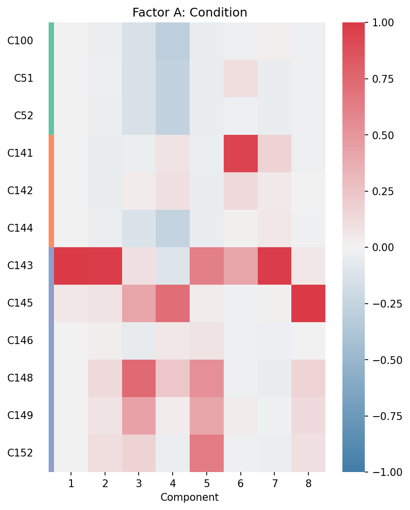
1. Factor A (Condition Factor): Shows how each experimental condition (e.g., patient sample, time point) contributes to each component

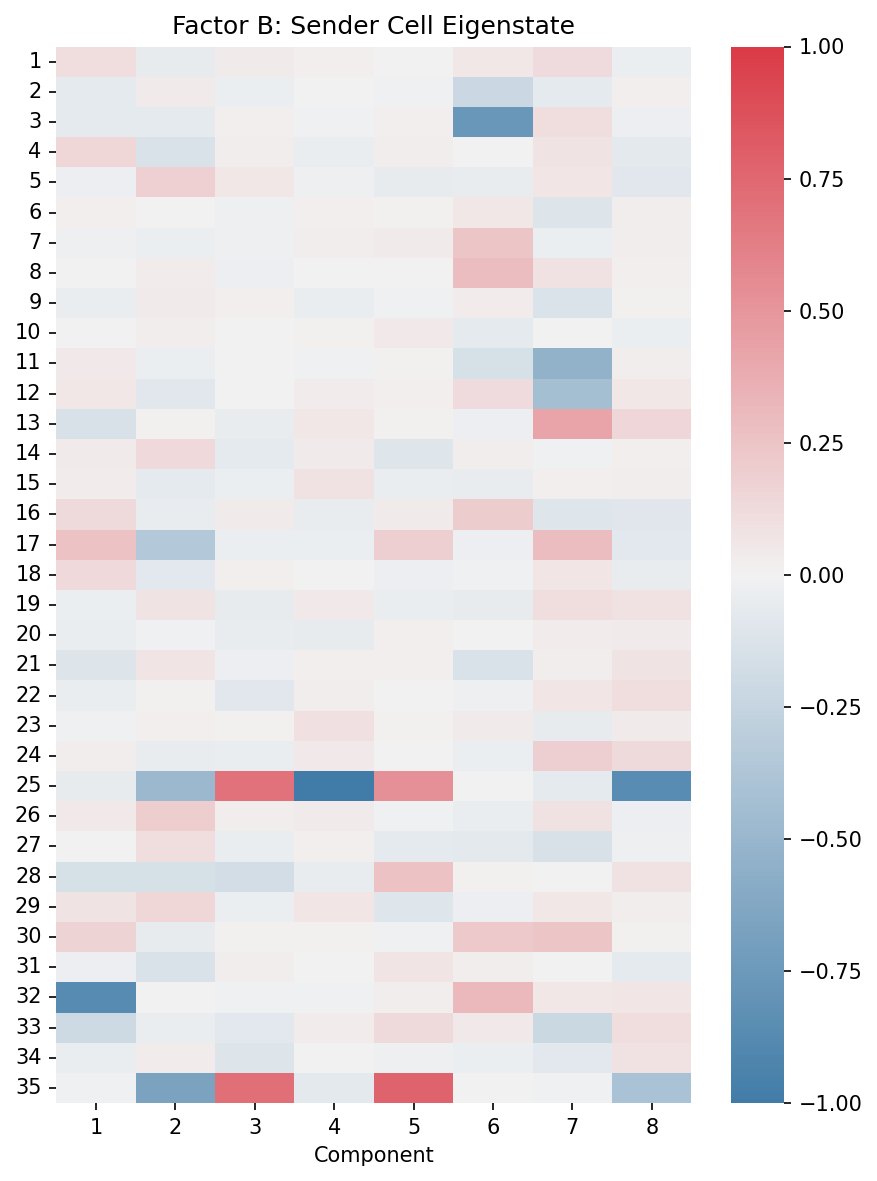
2. Factor B (Sender Cell Eigenstate): Represents sender cell patterns in the latent RISE space

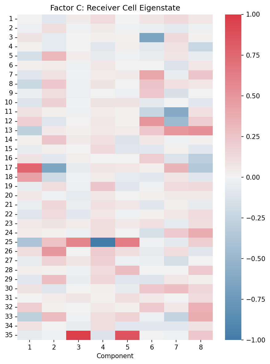
3. Factor C (Receiver Cell Eigenstate): Represents receiver cell patterns in the latent RISE space

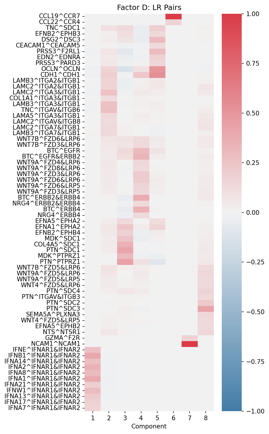
4. Factor D (Ligand-Receptor Pairs): Shows which L-R pairs drive each communication component

Visualize All Four Factors

Create visualizations for each of the four factor types:

from cellcommunicationpf2.figures.commonFuncs.plotFactors import (
    plot_condition_factors,
    plot_eigenstate_factors,
    plot_lr_factors
)
import matplotlib.pyplot as plt

# Prepare condition grouping (if you have multiple conditions per group)
condition_column = "sample"  # or your condition column name
group_col = "condition"      # optional: higher-level grouping

# Create mapping from samples to their condition groups
sample_to_group = X.obs.drop_duplicates(
    subset=[condition_column, group_col]
).set_index(condition_column)[group_col]

# Factor A: Condition factors
fig, ax = plt.subplots(figsize=(6, 8))
plot_condition_factors(
    X,
    ax,
    cond=condition_column,
    cond_group_labels=sample_to_group,
    group_cond=True,   # Sort by condition groups
    normalize=True     # Normalize each component
)
ax.set_title("Factor A: Condition")
plt.show()

# Factor B: Sender cell eigenstates
fig, ax = plt.subplots(figsize=(6, 8))
plot_eigenstate_factors(X, ax, factor_type="B")
ax.set_title("Factor B: Sender Cell Eigenstate")
plt.tight_layout()
plt.show()

# Factor C: Receiver cell eigenstates
fig, ax = plt.subplots(figsize=(6, 8))
plot_eigenstate_factors(X, ax, factor_type="C")
ax.set_title("Factor C: Receiver Cell Eigenstate")
plt.tight_layout()
plt.show()

# Factor D: Ligand-receptor pairs
fig, ax = plt.subplots(figsize=(6, 8))
plot_lr_factors(
    X,
    ax,
    trim=True,      # Show only top L-R pairs
    weight=0.08     # Threshold for inclusion
)
ax.set_title("Factor D: LR Pairs")
plt.tight_layout()
plt.show()

Understanding Each Factor

• Factor A (Condition): Heatmap rows represent conditions/samples, columns represent components. High values indicate which conditions are enriched in each communication pattern.

• Factor B (Sender Eigenstate): Heatmap shows sender cell patterns in the latent space. Each row is a latent dimension from RISE, each column is a CPD component.

• Factor C (Receiver Eigenstate): Similar to Factor B but for receiver cells. Reveals which latent receiver cell states participate in each component.

• Factor D (LR Pairs): Shows which ligand-receptor interactions drive each component. Only top-weighted pairs are displayed for clarity.

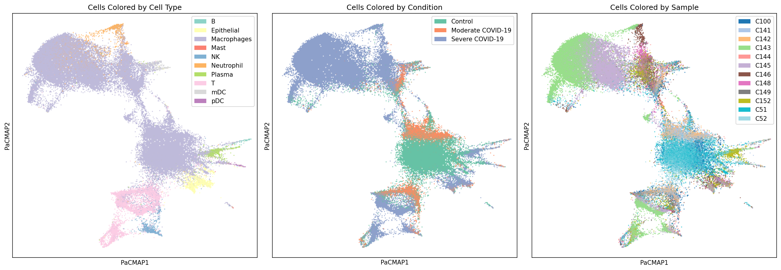
Visualize Cell Projections with PaCMAP

Explore how individual cells are positioned in the latent communication space:

from cellcommunicationpf2.figures.commonFuncs.plotPaCMAP import plot_labels_pacmap
import matplotlib.pyplot as plt
import seaborn as sns

# Create figure with 3 subplots
fig, axes = plt.subplots(1, 3, figsize=(18, 6))

# Plot colored by cell type
pal = sns.color_palette(palette="Set3")
pal = pal.as_hex()
plot_labels_pacmap(X, labelType="celltype", ax=axes[0], color_key=pal)
axes[0].set_title("Cells Colored by Cell Type")

# Plot colored by condition
pal = sns.color_palette("Set2")
pal = [pal[0], pal[1], pal[2]]
pal = [f"#{int(r*255):02x}{int(g*255):02x}{int(b*255):02x}" for r, g, b in pal]
plot_labels_pacmap(X, labelType="condition", ax=axes[1], color_key=pal)
axes[1].set_title("Cells Colored by Condition")

# Plot colored by sample
plot_labels_pacmap(X, labelType="sample", ax=axes[2])
axes[2].set_title("Cells Colored by Sample")

plt.tight_layout()
plt.show()

Interpreting a Component

Once you’ve identified components of interest, dig deeper into the specific cell types and ligand-receptor pairs driving the communication patterns.

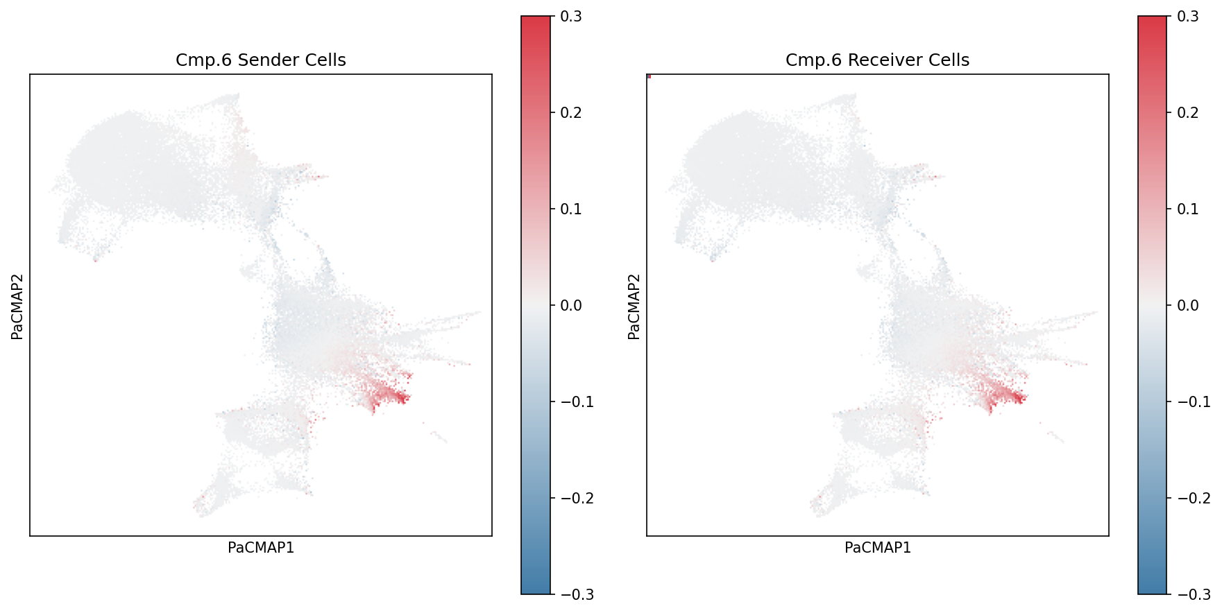
Visualize Specific Component Loadings

Use specialized plotting functions to visualize component weightings for a specific component:

from cellcommunicationpf2.figures.commonFuncs.plotPaCMAP import plot_wc_pacmap
import matplotlib.pyplot as plt

# Select component to visualize
component = 6

# Create figure with 2 subplots
fig, ax = plt.subplots(1, 2, figsize=(12, 6))

# Plot sender cell weightings
plot_wc_pacmap(X, component-1, ax[0], factor_matrix="B", cbarMax=0.3)
ax[0].set_title(f"Cmp.{component} Sender Cells")

# Plot receiver cell weightings
plot_wc_pacmap(X, component-1, ax[1], factor_matrix="C", cbarMax=0.3)
ax[1].set_title(f"Cmp.{component} Receiver Cells")

plt.tight_layout()
plt.show()

Violin Plots of Component Weights by Cell Type

Examine the distribution of component weights for specific cell types:

import seaborn as sns
import pandas as pd

# Select a component and cell type of interest
component = 6
cell_type = "mDC"

# Filter cells by cell type
X_celltype = X[X.obs["celltype"] == cell_type]

# Extract sender cell weights for this component
sender_weights = X_celltype.obsm["sc_B"][:, component-1]

# Create violin plot
fig, ax = plt.subplots(figsize=(6, 6))
sns.violinplot(data=sender_weights, ax=ax)
ax.set_ylim(-0.1, max(sender_weights) + 0.1)
ax.set_xlabel(f"{cell_type} Weight Distribution")
ax.set_ylabel(f"Sender Cell Component {component} Association")
ax.set_title(f"Distribution of Component {component} Weights in {cell_type}")
plt.tight_layout()
plt.show()

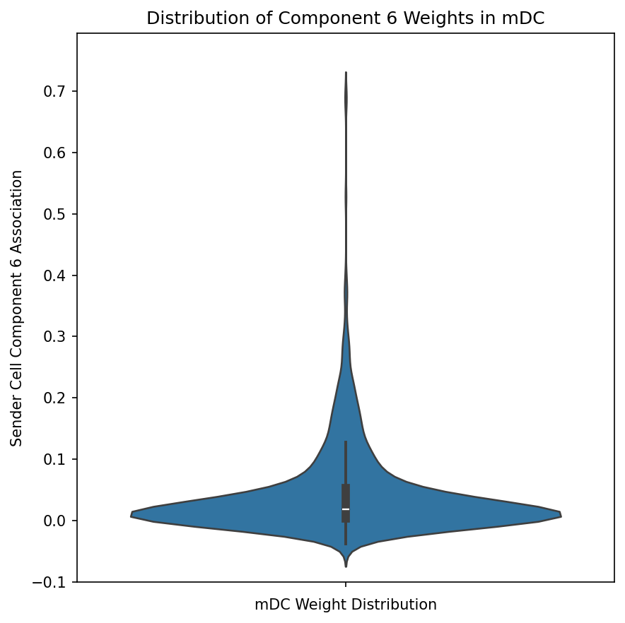
This visualization reveals whether a component is broadly active across all cells of a type or concentrated in a subset.

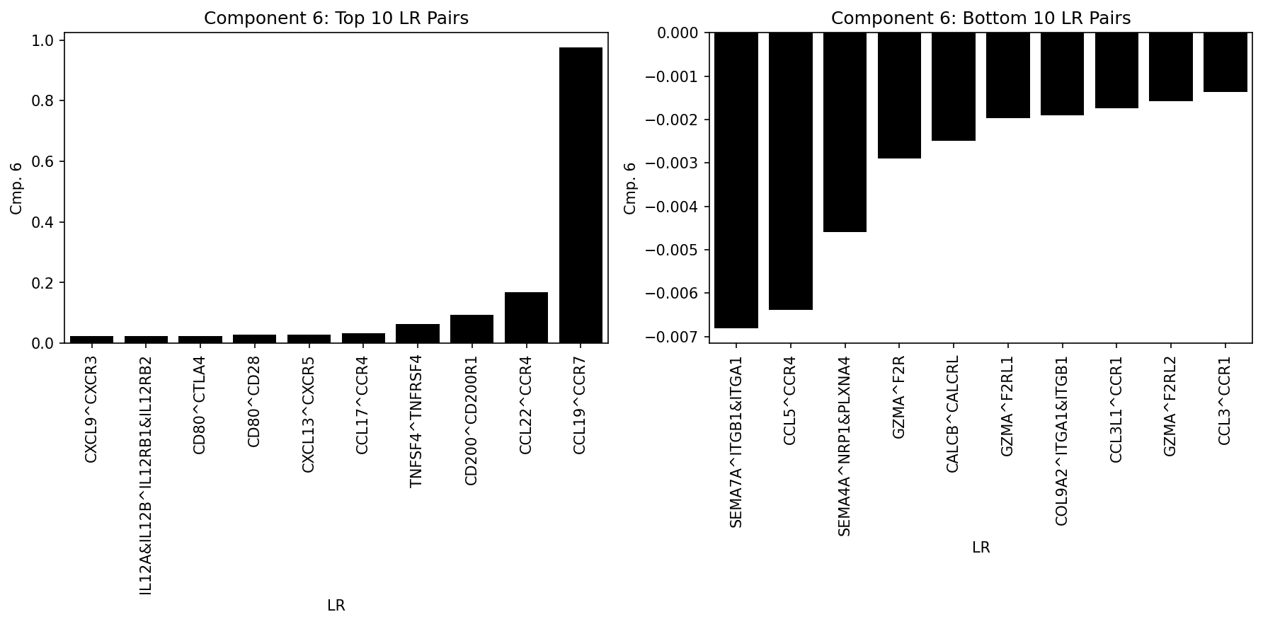
Analyze Top LR Pairs per Component

Visualize the most important ligand-receptor pairs for a specific component:

from cellcommunicationpf2.figures.commonFuncs.plotFactors import plot_lr_factors_partial
import matplotlib.pyplot as plt

cmp = 6
fig, ax = plt.subplots(1, 2, figsize=(12, 6))

# Plot top 10 LR pairs
plot_lr_factors_partial(X, cmp, ax[0], geneAmount=10, top=True)
ax[0].set_title(f"Component {cmp}: Top 10 LR Pairs")

# Plot bottom 10 LR pairs
plot_lr_factors_partial(X, cmp, ax[1], geneAmount=10, top=False)
ax[1].set_title(f"Component {cmp}: Bottom 10 LR Pairs")

plt.tight_layout()
plt.show()

Expression Product Heatmaps

Visualize the ligand-receptor expression products between sender and receiver cell populations to validate predicted interactions:

from cellcommunicationpf2.utils import (
    expression_product_matrix,
    average_product_matrix_ccc
)
import numpy as np
import seaborn as sns
import matplotlib.pyplot as plt

# Select component and L-R pair of interest
ccc_rise_cmp = 6
ligand = "CCL19"
receptor = "CCR7"

# Filter and sort sender cells by component weight
X_mdc_sender = X[X.obs["celltype"] == "mDC"]
X_mdc_sender = X_mdc_sender[np.argsort(-X_mdc_sender.obsm["sc_B"][:, ccc_rise_cmp-1])]

# Filter and sort receiver cells by component weight
X_mdc_receiver = X[X.obs["celltype"] == "mDC"]
X_mdc_receiver = X_mdc_receiver[np.argsort(X_mdc_receiver.obsm["rc_C"][:, ccc_rise_cmp-1])]

# Calculate expression product matrix for mDC -> mDC
df = expression_product_matrix(X_mdc_sender, X_mdc_receiver, ligand, receptor)
df = average_product_matrix_ccc(df)

# Create heatmap
fig, ax = plt.subplots(figsize=(6, 6))
sns.heatmap(df, ax=ax, cmap="viridis", vmax=0.12)
ax.set_xlabel("Receiver mDCs")
ax.set_ylabel("Sender mDCs")
ax.set_title("CCL19-CCR7 Interaction")
ax.set_xticks([])
ax.set_yticks([])
plt.tight_layout()
plt.show()

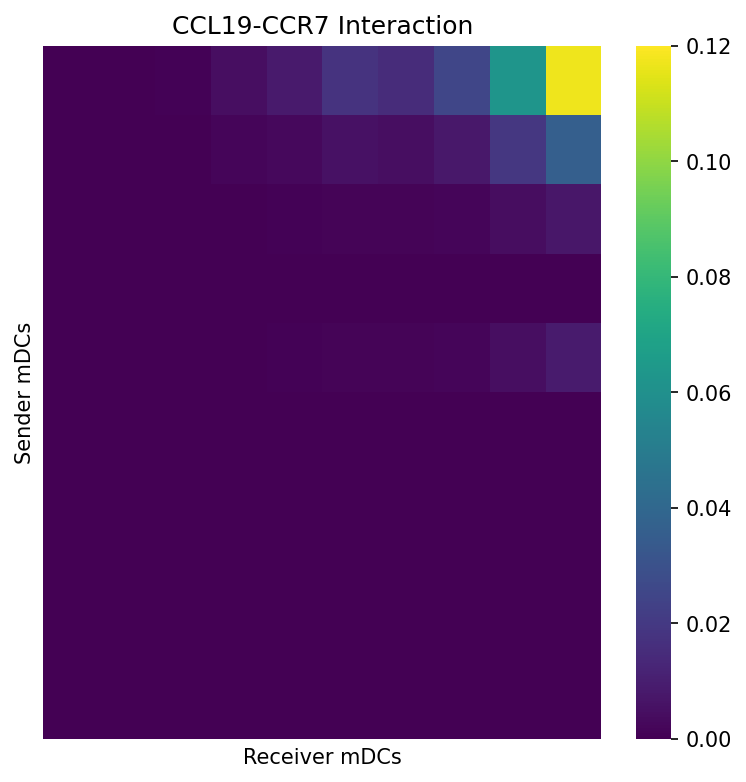
This heatmap shows the product of ligand expression (in senders) and receptor expression (in receivers), revealing which cell pairs have the highest potential for this specific interaction.